On 27 September 2024, Helene’s remnants dumped over a foot of rain across the southern Appalachians. The Swannanoa and French Broad rivers tore through Asheville, NC. Whole neighborhoods — Biltmore Village, the River Arts District, the Swannanoa corridor — went under several meters of water. Hundreds died.
Two questions a humanitarian coordinator might ask, looking at the same map:
Which buildings were inundated? And how deeply?
How many people, how many hospitals?
Below is a map and a small dashboard that answers both, interactively. Drag the slider — the buildings shown filter by flood depth. The map and stats update live; no Python kernel is running underneath this page.
import sys, pathlib, json
ROOT = pathlib.Path("..").resolve() if pathlib.Path("..").exists() else pathlib.Path("../..").resolve()
sys.path.insert(0, str(ROOT))
import numpy as np
import pandas as pd
import geopandas as gpd
import matplotlib.pyplot as plt
from shapely.geometry import Polygon, Point, shape
import lonboard
from lonboard import Map, ScatterplotLayer, PolygonLayer, BitmapLayer
from widgets.hurricane_dashboard.widget import HurricaneDashboard
DATA = ROOT / "data" / "helene"
print("data dir:", DATA)
data dir: /Users/sanjay/seed/anywidget-experiments/data/helene
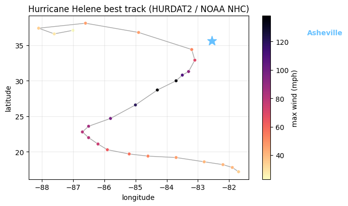
Step 1 — Helene’s track from HURDAT2
NOAA’s HURDAT2 best-track file contains every Atlantic storm since 1851. We extract Helene (AL092024) and plot her path. By the time she crossed into North Carolina she’d weakened considerably from her Cat 4 landfall in Florida — the headline in NC was rain, not wind.
def parse_hurdat2(path):
rows = []
with open(path) as f:
cur_id = cur_name = None
for line in f:
parts = [p.strip() for p in line.strip(", \n").split(",")]
if parts and parts[0].startswith("AL") and len(parts) == 3:
cur_id, cur_name = parts[0], parts[1]
continue
if not cur_id or len(parts) < 8:
continue
try:
rows.append({
"storm_id": cur_id,
"name": cur_name,
"date": parts[0],
"time": parts[1],
"lat": float(parts[4][:-1]) * (1 if parts[4][-1] == "N" else -1),
"lon": float(parts[5][:-1]) * (-1 if parts[5][-1] == "W" else 1),
"wind_kt": int(parts[6]),
"pressure_mb": int(parts[7]) if parts[7] != "-999" else np.nan,
})
except (ValueError, IndexError):
continue
return pd.DataFrame(rows)
storms = parse_hurdat2(DATA / "hurdat2.txt")
helene = storms[storms.storm_id == "AL092024"].copy()
helene["wind_mph"] = helene["wind_kt"] * 1.151
print(f"{len(helene)} track points; peak wind {helene.wind_mph.max():.0f} mph")
helene.head()
25 track points; peak wind 138 mph
fig, ax = plt.subplots(figsize=(7, 4.2))
sc = ax.scatter(helene.lon, helene.lat, c=helene.wind_mph, cmap="magma_r",
s=22, edgecolor="white", linewidth=0.4)
ax.plot(helene.lon, helene.lat, color="0.4", linewidth=1, alpha=0.6, zorder=0)
# Asheville reference point
ax.plot(-82.55, 35.59, marker="*", color="#67c1ff", markersize=14, zorder=5)
ax.annotate("Asheville", xy=(-82.55, 35.59), xytext=(-79.5, 36.5),
color="#67c1ff", fontsize=10, fontweight="bold")
plt.colorbar(sc, ax=ax, label="max wind (mph)")
ax.set_xlabel("longitude"); ax.set_ylabel("latitude")
ax.set_title("Hurricane Helene best track (HURDAT2 / NOAA NHC)")
ax.grid(alpha=0.25)
plt.tight_layout()
plt.show()
Step 2 — load Asheville buildings + hospitals from OSM
The OpenStreetMap extract is fetched at prebuild time by data/helene/fetch.py
(via the Overpass API for a ~10 × 10 km bbox around Asheville). For our purposes
each building reduces to a centroid — enough to light up the map with thousands
of dots without shipping every polygon.
def load_osm_ways(path, kind):
"""Return a GeoDataFrame with one row per way (polygon) or node (point)."""
with open(path) as f:
data = json.load(f)
rows = []
for el in data["elements"]:
if el["type"] == "way" and "geometry" in el:
ring = [(g["lon"], g["lat"]) for g in el["geometry"]]
if len(ring) >= 3:
try:
poly = Polygon(ring)
if poly.is_valid and poly.area > 0:
rows.append({"id": el["id"], "geometry": poly,
"tags": el.get("tags", {})})
except Exception:
pass
elif el["type"] == "node":
rows.append({"id": el["id"], "geometry": Point(el["lon"], el["lat"]),
"tags": el.get("tags", {})})
gdf = gpd.GeoDataFrame(rows, crs="EPSG:4326")
return gdf
bldgs = load_osm_ways(DATA / "osm_buildings.json", "building")
hosps = load_osm_ways(DATA / "osm_hospitals.json", "hospital")
print(f"{len(bldgs):,} buildings, {len(hosps):,} hospitals")
# Centroids for fast map rendering
bldgs["centroid"] = bldgs.geometry.centroid
41,037 buildings, 3 hospitals
/var/folders/d9/k5r736hx3gvf5q7pw2g1lz680000gn/T/ipykernel_9874/2573587109.py:28: UserWarning: Geometry is in a geographic CRS. Results from 'centroid' are likely incorrect. Use 'GeoSeries.to_crs()' to re-project geometries to a projected CRS before this operation.
bldgs["centroid"] = bldgs.geometry.centroid
Step 3 — flood polygon, point-in-polygon to assign depths
The flood polygons in data/helene/flood_extent.geojson are a hand-authored
approximation of the Swannanoa / French Broad valleys (a proper analysis would
use Sentinel-1 SAR-derived inundation extent — Copernicus EMS rapid mapping
product EMSR755 covered the region). Each polygon carries an estimated water
depth. We sjoin building centroids to the polygons and tag each building with
the depth at its location (or 0 if outside any polygon).
flood = gpd.read_file(DATA / "flood_extent.geojson")
print(f"{len(flood)} flood polygons; depths {sorted(flood.depth_m.unique())} m")
# sjoin building centroids onto flood polygons
cent_gdf = gpd.GeoDataFrame(bldgs[["id"]].copy(), geometry=bldgs["centroid"], crs="EPSG:4326")
joined = gpd.sjoin(cent_gdf, flood[["depth_m", "geometry"]], how="left", predicate="within")
# Where a building falls in multiple overlapping polygons, take the deepest
depth_per_building = joined.groupby("id")["depth_m"].max().fillna(0.0)
bldgs["flood_depth_m"] = bldgs["id"].map(depth_per_building).fillna(0.0)
print("flooded buildings:", int((bldgs.flood_depth_m > 0).sum()))
print("max depth assigned:", float(bldgs.flood_depth_m.max()))
5 flood polygons; depths [np.float64(0.4), np.float64(0.6), np.float64(1.6), np.float64(3.4), np.float64(4.2)] m
flooded buildings: 8024
max depth assigned: 4.2
Step 4 — bucket buildings by depth, aggregate stats
Four buckets:
| Bucket | Depth | Color |
|---|---|---|
dry | 0 m | grey |
shallow | 0 < d ≤ 1 m | yellow |
deep | 1 < d ≤ 3 m | orange |
drowned | d > 3 m | red |
Stats are precomputed per slider position so the JS just looks them up.
def bucket(d):
if d <= 0: return "dry"
if d <= 1: return "shallow"
if d <= 3: return "deep"
return "drowned"
bldgs["bucket"] = bldgs["flood_depth_m"].map(bucket)
counts = bldgs["bucket"].value_counts().reindex(["dry", "shallow", "deep", "drowned"], fill_value=0)
print(counts)
# Hospitals affected = those whose centroid is in the flood polygon
hosp_pts = gpd.GeoDataFrame(hosps[["id", "tags"]].copy(),
geometry=hosps.geometry.centroid,
crs="EPSG:4326")
hosp_joined = gpd.sjoin(hosp_pts, flood[["geometry"]], how="left", predicate="within")
hospitals_affected = int(hosp_joined["index_right"].notna().sum())
# Rough population estimate: 2.4 people per residential building (urban avg).
PEOPLE_PER_BLDG = 2.4
# Threshold semantics: 0 = show everything, 1 = ≥shallow, 2 = ≥deep, 3 = drowned only
threshold_layer_map = [
["b_dry", "b_shallow", "b_deep", "b_drowned"],
["b_shallow", "b_deep", "b_drowned"],
["b_deep", "b_drowned"],
["b_drowned"],
]
stats_tables = []
for buckets in threshold_layer_map:
name_to_count = {f"b_{b}": int(counts.get(b, 0)) for b in counts.index}
visible_buildings = sum(name_to_count.get(k, 0) for k in buckets)
# Hospitals only count as "affected" if any flooded layer is on
hosp_count = hospitals_affected if any(k != "b_dry" for k in buckets) else 0
# People estimate: same buildings × ratio, but only flooded ones contribute
flooded_visible = sum(name_to_count.get(k, 0) for k in buckets if k != "b_dry")
stats_tables.append({
"buildings": visible_buildings,
"hospitals": hosp_count,
"people_est": int(flooded_visible * PEOPLE_PER_BLDG),
})
stats_tables
bucket
dry 33013
shallow 2957
deep 1606
drowned 3461
Name: count, dtype: int64
/var/folders/d9/k5r736hx3gvf5q7pw2g1lz680000gn/T/ipykernel_9874/345491478.py:13: UserWarning: Geometry is in a geographic CRS. Results from 'centroid' are likely incorrect. Use 'GeoSeries.to_crs()' to re-project geometries to a projected CRS before this operation.
geometry=hosps.geometry.centroid,
[{'buildings': 41037, 'hospitals': 2, 'people_est': 19257},
{'buildings': 8024, 'hospitals': 2, 'people_est': 19257},
{'buildings': 5067, 'hospitals': 2, 'people_est': 12160},
{'buildings': 3461, 'hospitals': 2, 'people_est': 8306}]Step 5 — assemble the map and dashboard
We make one ScatterplotLayer per bucket so the dashboard can hide/show layers
by toggling the visible trait — much simpler than per-feature color updates
through Arrow buffers. Hospitals get their own layer, the flood polygon is a
PolygonLayer, the post-storm MODIS image becomes a BitmapLayer underneath.
The dashboard widget knows nothing about any of these directly. We hand it
a dict of {layer_key → layer.model_id} plus the precomputed threshold/stats
tables. In the browser it uses host.waitForModel() to resolve each layer
by UUID and toggles visible. The widget renders sticky so it stays in view
as you scroll the map.
import base64
def png_to_data_url(path):
return "data:image/png;base64," + base64.b64encode(path.read_bytes()).decode()
def safe_layer(points, color, radius=14):
"""ScatterplotLayer that tolerates empty buckets by inserting a phantom
point off the visible map. Lonboard's geoarrow conversion can't handle a
truly empty geometry list."""
if len(points) == 0:
points = gpd.GeoSeries([Point(0, 0)], crs="EPSG:4326")
geom = gpd.GeoDataFrame(geometry=gpd.GeoSeries(points.values, crs="EPSG:4326"))
return ScatterplotLayer.from_geopandas(
geom, get_fill_color=color, get_radius=radius,
radius_min_pixels=1.5, opacity=0.85,
)
# Layers (each is a separate lonboard layer with its own model_id)
bitmap_after = BitmapLayer(
image=png_to_data_url(DATA / "modis_after.png"),
bounds=[-82.70, 35.45, -82.40, 35.72], # west, south, east, north
opacity=0.55,
)
flood_layer = PolygonLayer.from_geopandas(
flood,
get_fill_color=[80, 160, 235, 110],
get_line_color=[80, 160, 235, 220],
line_width_min_pixels=1,
)
def bucket_centroids(name):
return bldgs.loc[bldgs.bucket == name, "centroid"]
building_layers = {
"b_dry": safe_layer(bucket_centroids("dry"), [110, 110, 110, 160], 8),
"b_shallow": safe_layer(bucket_centroids("shallow"), [255, 220, 80, 240], 16),
"b_deep": safe_layer(bucket_centroids("deep"), [255, 140, 60, 240], 20),
"b_drowned": safe_layer(bucket_centroids("drowned"), [220, 50, 50, 250], 24),
}
hosp_layer = ScatterplotLayer.from_geopandas(
gpd.GeoDataFrame(geometry=gpd.GeoSeries(hosp_pts.geometry.values, crs="EPSG:4326")),
get_fill_color=[230, 80, 200, 250],
get_radius=80,
radius_min_pixels=6,
stroked=True,
get_line_color=[255, 255, 255, 255],
line_width_min_pixels=2,
)
m = Map(
layers=[bitmap_after, flood_layer,
building_layers["b_dry"], building_layers["b_shallow"],
building_layers["b_deep"], building_layers["b_drowned"],
hosp_layer],
view_state={"longitude": -82.555, "latitude": 35.585, "zoom": 12.5, "pitch": 0, "bearing": 0},
show_tooltip=False,
)
layer_uuids = {
"modis_after": bitmap_after.model_id,
"flood": flood_layer.model_id,
"b_dry": building_layers["b_dry"].model_id,
"b_shallow": building_layers["b_shallow"].model_id,
"b_deep": building_layers["b_deep"].model_id,
"b_drowned": building_layers["b_drowned"].model_id,
"hospitals": hosp_layer.model_id,
}
dashboard = HurricaneDashboard(
layer_uuids=layer_uuids,
initial_visible={
"modis_after": True,
"flood": True,
"hospitals": True,
# building layers are controlled by the threshold, default = all visible
"b_dry": True, "b_shallow": True, "b_deep": True, "b_drowned": True,
},
toggle_layers=[
{"key": "modis_after", "label": "Satellite (MODIS post-storm)"},
{"key": "flood", "label": "Flood extent"},
{"key": "hospitals", "label": "Hospitals"},
],
threshold_layer_map=threshold_layer_map,
stats_tables=stats_tables,
threshold=0,
)
print(f"map: {len(m.layers)} layers · dashboard: {len(layer_uuids)} layer bindings")
map: 7 layers · dashboard: 7 layer bindings
The map and the dashboard
Drag the slider in the dashboard — the map below filters to buildings at that flood depth or worse, and the counters retween. Toggle the satellite, flood-extent, and hospitals layers from the dashboard checkboxes. The dashboard floats sticky on the right so you can keep adjusting controls while you scroll the map.
from IPython.display import display
display(dashboard)
display(m)
Sources:
HURDAT2 best-track — NOAA NHC, public.
Buildings + hospitals — OpenStreetMap via Overpass.
MODIS Terra true-color — NASA GIBS, public.
Flood polygon — hand-authored stand-in for Copernicus EMS EMSR755.
People estimate uses a generic urban occupancy ratio of 2.4 / residential building.