A small interactive that walks 144 years of US baby-name data (1880–2023, courtesy of the Social Security Administration) and lets you watch any name rise, peak, and fade. Type your name. The chart sweeps from 1880 to today; you’ll see when your name was its most popular, and which other names rose and fell with it.
The Python here is the boring serious part — load CSVs, normalize, find nearest-trajectory neighbors. The fun part is in the JS widget at the bottom.
import sys, pathlib
ROOT = pathlib.Path("..").resolve() if pathlib.Path("..").exists() else pathlib.Path("../..").resolve()
sys.path.insert(0, str(ROOT))
import numpy as np
import pandas as pd
import matplotlib.pyplot as plt
from widgets.name_explorer.widget import NameExplorer
DATA = ROOT / "data" / "names"
print("data dir:", DATA)
print("yob files:", len(list(DATA.glob("yob*.txt"))))
data dir: /Users/sanjay/seed/anywidget-experiments/data/names
yob files: 144
Step 1 — load 144 years of CSVs
Each yob{year}.txt is a three-column CSV: name, sex, count. We concat them all
into one tidy DataFrame and add a year column.
frames = []
for path in sorted(DATA.glob("yob*.txt")):
year = int(path.stem.replace("yob", ""))
df = pd.read_csv(path, names=["name", "sex", "count"])
df["year"] = year
frames.append(df)
raw = pd.concat(frames, ignore_index=True)
print(f"{len(raw):,} rows across {raw.year.nunique()} years")
raw.head()
2,117,219 rows across 144 years
Step 2 — pivot to a (name|sex) × year matrix, top 5,000 by lifetime count
Cap at 5,000 names to keep the page light and the cosine-similarity matrix small. That covers the names ~99% of US-born people would search for; rarer names are silently absent.
raw["key"] = raw["name"] + "|" + raw["sex"]
YEAR_START, YEAR_END = 1880, int(raw["year"].max())
years = list(range(YEAR_START, YEAR_END + 1))
totals = raw.groupby("key")["count"].sum().sort_values(ascending=False)
TOP_N = 5000
top_keys = totals.head(TOP_N).index.tolist()
mat = (
raw[raw["key"].isin(top_keys)]
.pivot_table(index="key", columns="year", values="count", fill_value=0, aggfunc="sum")
.reindex(index=top_keys, columns=years, fill_value=0)
.astype(np.int32)
)
print("matrix shape:", mat.shape)
mat.head()
matrix shape: (5000, 144)
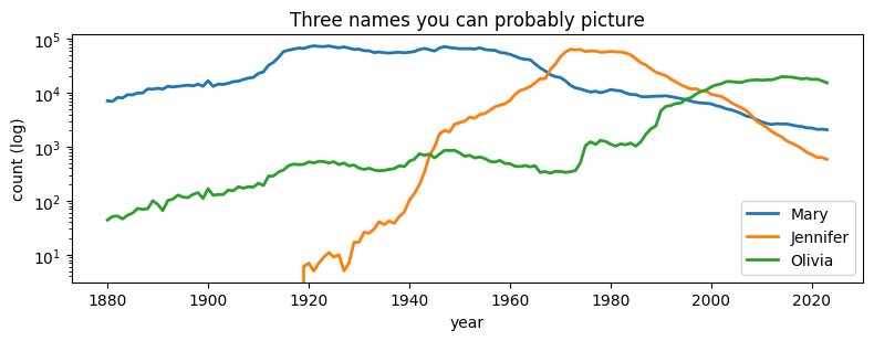
Step 3 — what does a trajectory look like?
Just one static plot for context, then we hand off to the interactive widget.
fig, ax = plt.subplots(figsize=(8, 3.2))
for k in ["Mary|F", "Jennifer|F", "Olivia|F"]:
if k in mat.index:
ax.plot(years, mat.loc[k].values, label=k.split("|")[0], linewidth=2)
ax.set_yscale("log")
ax.set_xlabel("year")
ax.set_ylabel("count (log)")
ax.legend()
ax.set_title("Three names you can probably picture")
plt.tight_layout()
plt.show()
Step 4 — find each name’s peak year and rank
The widget shows a “peaked in 1921 · #1” pill. We compute year-of-max-count and the within-year rank by sex.
# Year-of-max per name
peak_year = mat.values.argmax(axis=1)
peak_count = mat.values.max(axis=1)
peak_year_actual = np.array(years)[peak_year]
# Within-year rank by sex (1 = most popular for that sex that year)
rank_lookup = {}
for yr, sub in raw.groupby("year"):
for sex, sub2 in sub.groupby("sex"):
order = sub2.sort_values("count", ascending=False).reset_index(drop=True)
rank_lookup[(yr, sex)] = {
row["name"]: idx + 1 for idx, row in order.iterrows()
}
peaks = {}
for i, key in enumerate(mat.index):
name, sex = key.split("|")
yr = int(peak_year_actual[i])
rank = rank_lookup.get((yr, sex), {}).get(name, None)
peaks[key] = {
"year": yr,
"rank": int(rank) if rank else 0,
"count": int(peak_count[i]),
}
list(peaks.items())[:3]
[('James|M', {'year': 1947, 'rank': 1, 'count': 94761}),
('John|M', {'year': 1947, 'rank': 3, 'count': 88320}),
('Robert|M', {'year': 1947, 'rank': 2, 'count': 91654})]Step 5 — trajectory twins via cosine similarity on z-scored shapes
We z-score each name’s series (subtract mean, divide by std) so that “Mary’s” and “Margaret’s” similarity captures shape, not magnitude. Then cosine similarity on the normalized matrix; top 4 nearest per name.
X = mat.values.astype(np.float32)
mu = X.mean(axis=1, keepdims=True)
sd = X.std(axis=1, keepdims=True)
sd[sd == 0] = 1.0
Z = (X - mu) / sd
# unit-normalize rows for cosine
norms = np.linalg.norm(Z, axis=1, keepdims=True)
norms[norms == 0] = 1.0
Zn = (Z / norms).astype(np.float32)
# Cosine matrix and top-K — done in chunks to be memory-friendly. We
# also drop pairs where the bare name (sans sex) matches the source,
# so "Jennifer F" doesn't list "Jennifer M" as its twin.
K = 4
n = Zn.shape[0]
keys = mat.index.tolist()
bare = [k.split("|")[0].lower() for k in keys]
twins = {}
chunk = 1000
for start in range(0, n, chunk):
sim = Zn[start : start + chunk] @ Zn.T # (chunk, n)
for i in range(sim.shape[0]):
sim[i, start + i] = -np.inf
# Mask other-sex pairings of the same bare name
same = bare[start + i]
for j, b in enumerate(bare):
if b == same:
sim[i, j] = -np.inf
# Pull a few extra candidates so we have headroom after masking
cand = np.argpartition(-sim, K + 2, axis=1)[:, : K + 2]
for i in range(sim.shape[0]):
row_idx = cand[i]
order = np.argsort(-sim[i, row_idx])
twins[keys[start + i]] = [keys[j] for j in row_idx[order][:K]]
print("twin lookup built for", len(twins), "names")
twins["Mary|F"]
twin lookup built for 5000 names
['Martha|F', 'Ralph|M', 'Willie|M', 'Howard|M']Step 6 — package up for the widget
Trajectories ship as plain int arrays keyed by Name|Sex. Era captions come
from a hand-curated CSV in data/names/. Widget state ends up around 2–3 MB.
trajectories = {key: mat.loc[key].astype(int).tolist() for key in mat.index}
era_df = pd.read_csv(DATA / "era_captions.csv")
era_captions = {str(int(r.decade)): r.caption for r in era_df.itertuples()}
name_index = sorted(mat.index.tolist(), key=lambda k: (k.split("|")[0].lower(), k.split("|")[1]))
print(f"trajectories: {len(trajectories):,} · twins: {len(twins):,} · peaks: {len(peaks):,}")
print(f"era captions: {list(era_captions.items())[:2]} ...")
trajectories: 5,000 · twins: 5,000 · peaks: 5,000
era captions: [('1880', 'the gilded age — Mary, John, William ruled'), ('1890', 'close of the frontier; Helen and Charles rose')] ...
Step 7 — render
Type a name. Hit enter (or pick from the dropdown). Try Claude for a small
surprise. Optionally type a birth year to anchor the chart.
widget = NameExplorer(
trajectories=trajectories,
peaks=peaks,
twins=twins,
era_captions=era_captions,
name_index=name_index,
selected="Mary|F",
year_start=YEAR_START,
year_end=YEAR_END,
)
widget
Data: Social Security Administration, public-domain.
Widget code in widgets/name_explorer/. The interactive page you’re looking at
is built statically — no Python kernel running underneath.